Economically Optimal Inventory

This article was published in APICS Extra, Vol 4, No. 10, October 28, 2009 : Author Pankaj Mehta

Summary

In this paper we explore the consequences of maintaining different stock levels under varying demand conditions and arrive at a simple formula for calculating the economically optimum stock level. The result is a surprisingly elegant formula that may be confidently applied by practitioners to set their inventory levels.

Problem

The problem that we are going to solve can be stated as follows:

Given that the demand for a stock keeping unit is normally distributed with average demand μ and standard deviation σ, what is the optimum stock level considering financial attributes: Price P, Cost C and Inventory holding cost of I%.

In such a situation, it is usual and convenient for inventory managers to set the stock equal to μ + z σ. The variable z is generally set based on some simple business rules and is at times arrived at indirectly by selecting a service level (cumulative normal probability distribution function). The only thing in favour of this practice is its simplicity. The biggest problem of course is that the decision process is not rooted in economics and businesses might potentially be losing money by tying it up in unnecessary inventory.

Modelling Sales

The current state of affairs has arisen not because of neglect but because of the difficulties involved in carrying out a proper mathematical analysis.

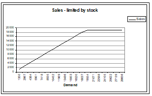
It is obvious that if there is unlimited amount of stock on hand then the sales will equal the underlying demand. If stock is limited then the sales will be limited to the amount of stock, as is illustrated by the figure below.

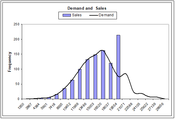
If there were a known way of estimating the sales under different scenarios then it would open the way to the determination of an optimum. Our approach was to simulate demand to arrive at the corresponding sales. The next figure represents the results of the simulation – the continuous curve is spread of the demand (approximates the bell shaped curve) and the histogram is the spread of sales. As expected, there are no sales larger than the stock on hand and none greater than the underlying demand. This example is based on stock level corresponding to z=1 and what was surprising was the fact that the expected sale came up to 98% of the underlying demand. Without the benefit of the simulation one would have been tempted to think that the sales would be somewhat but not a lot more than 85%.

Curious as we were to see whether the above was a one off result peculiar to the chosen parameters, we ran simulations for different values of standard deviations and for different values of z. The results are shown in the following chart.

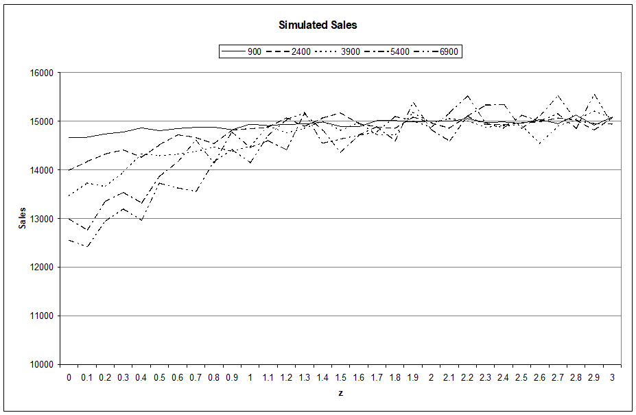
As z increases, no matter what the standard deviation is, the average sale tends to approach the average sale. For lower levels of z, the curves tend to diverge and the divergence is related to the standard deviation. Based on the shape of the curve and after carrying out regression analyses we have been able to arrive at an empirical formula that can be used to predict the sales without the need for slow and expensive simulations. That formula is:

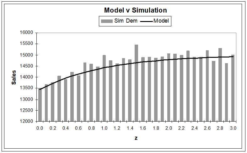
Expected Sale = μ (1 – 0.4 σ/μ exp(-z))

The degree of fit provided by this formula can be gauged from the following chart.

Optimisation

As stock is increased, sales and profits will increase but there will come a point when the marginal increase in profit would be less than the increase in inventory holding cost. There would be no point in increasing stock any further.

Expected revenue = μ (1 – 0.4 σ/μ exp(-z)) (P-C)

Rate of change of expected revenue = 0.4 σ(P-C) exp(-z)

Inventory holding cost = (μ/2 + (μ+ z σ) C I

Rate of change of inventory holding cost = σ C I

From the above, it follows that the optimum z = - ln (2.5 C I / (P – C))

Of course, the same result could have been arrived at by noting that the net profit would be maximum at a point where its derivative is zero.

Conclusion

We have arrived at a simple empirical formula that can be confidently applied to arrive at economically optimal stock levels. It depends solely on the financial parameters and being easy to work out can be used as and when prices and costs are updated to ensure that inventory never turns towards uneconomical levels.

However, it should be noted that what is economically optimum may not be commercially the best answer. For example, if the business has guaranteed that there will never be stock-outs of a certain item then the stocks would have be to kept at higher levels – but now you would know what the price of that guarantee is.